Conjugate Gradient Method in Solving Linear Equation System

Linear Equation System

In fluid simulation, sometimes we need to solve a Linear Equation System like doing projection in Eulerian fluid. A linear Equation System can be written as a matrix form: $$ Ax = b $$

where $A$ is a $N\times N$ matrix and $x,b$ are $N\times 1$ vectors. Actually, we have a lot of methods to solve this problem, like Gauss-Seidel iteration, Gaussian elimination, etc. When simulating fluid, we always use Conjugate Gradient to solve linear system because it’s more quick than other methods.

Convert Solving to Optimizing

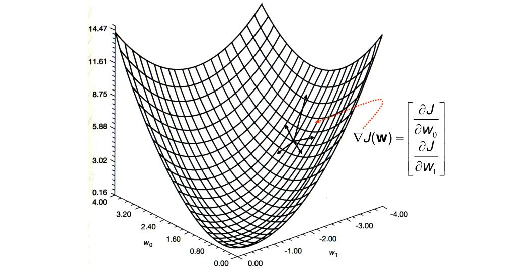
A really important fact is that if matrix $A$ is a symmetrical matrix, we can consider solving the equation as a mission to find the minimun value of function: $$ f(x) = \frac{1}{2}x^TAx - bx $$

To find the minimum value, we can guess a value at first, which is $x_0$ . Then use negative gradient as the dirction we will step and step to the lowest point, which is $x_1$. Iterate this loop again and again, we will get lower and lower in the valley and finally we will get the lowest position. This method is “steepest descent method”.

In steepest descent method, every time we use $$ -\nabla f = b - Ax_i $$ as the direction to step. It’s an intuitive choice, but we can find some better direction in global aspect.

A-orthogonal

In linear algebra, we define the dot product of two vectors as: $$ (a, b) = a\cdot b = a^Tb $$

if $(a,b) = 0$ , we say $a$ and $b$ are orthogonal. Now, we define “A-orthogonal”. We say $a$ and $b$ are A-orghogonal if $$ (a,b)^A = a^TAb = 0 $$

With A-orthogonal vectors ${a_1, …, a_n}$ , we can easily find the represent of solution $x$ in such a base: $$ x = \sum_{k=1}^n \frac{(a_k, b)}{(a_k, a_k)^A} a_k $$

So the problem is: how to find the A-orthogonal vectors? If you’re good at linear algebra, you might say finding the eigen vectors of A. But it’s not a good idea because calculating eigen vectors is even more difficult than solving the equations. So, we choose to generate them dynamically :

1. First, we can give an arbitrary vector as $a_1$.

2. To generate $a_2$, we choose an arbitrary vector $t_2$ which is not parallel with $a_1$ . Then we can get $a_1$ by: $$ a_1 = t_2 - \frac{(t_2, a_1)^A}{(a_1, a_1)^A} a_1 $$

3. For $a_k$, we have an arbitrary vector $t_k$ which is not parallel with $a_i (1\leq i < k)$ . Then we have :

$$ a_k = t_k - \sum_{i=1}^{k-1} \frac{(t_k, a_i)^A}{(a_i, a_i)^A} a_i $$

In fact, method above is a Gram–Schmidt process in A-orthogonal. But it’s not efficient enough in solving the linear equation, we can even make it better.

Conjugate Gradient Method

In last section, we generate $t_k$ randomly in every iteration. But if we combine it with deepest descent method, we can have a better verison. If we use $-\nabla f = b - Ax_{k-1}$ as $t_k$ , we can prove (by induction) that: $$ a_k = t_k - \frac{(t_k, a_{k-1})^A}{(a_{k-1}, a_{k-1})^A} a_{k-1} $$

is A-orthogonal with $a_i (1\leq i < k)$ , where $x_{k-1}$ is:

$$ x = \sum_{i=1}^{k-1} \frac{(a_i, b)}{(a_i, a_i)^A} a_i $$

which means we don’t need to run the loop to find the $a_k$ .

Now, we have the algrithm for CG :

1
2
3
4
5
6
7
8
9

have a initial guess x
t = b - A * x
a = t
x = a.dot(b) / a.Adot(a) * a

for i in range(n) :
    t = b - A * x
    a = t - t.Adot(a) / a.Adot(a) * a
    x += a.dot(b) / a.dot(a) * a

looks good, right? So why did I mention the deepest descent method? The truth is, if you read this code carefully, you will find that it’s almost same as the code for deepest descent method. The only difference is in deepest descent method we use $t_i = b - A * x_i$ as step direction but in CG we use $a_i$ , which is computed from $t_i$ .

Summarize

Right now, we have two different aspects to see the CG method:

1. We need to find $n$ vectors that are A-orthogonal with each other. If we choose $t_k$ smartly, we can avoid the loop.

2. In steepest descent method, using $-\nabla f$ as direction is not good enough. We can choose a direction that is A-orthogonal with all directions we’ve steped before. In this method we will have at most $n$ steps to destination.

Actually, in practice we don’t need to run all $n$ loops. At most time if $b - Ax$ is small enough we can break the loop. If $A$ is ill-conditioned, we will have more steps to make it small enough, so we have some pre-conditioner to make matrix $A$ more “health”.

Reference:

• An Introduction to the Conjugate Gradient Method Without the Agonizing Pain

• An English video : Youtube

• A Mandarin video from Soochow University : Bilibili